Sequence data contamination from biological or digital sources can obscure true results and falsely raise one’s hopes. Contamination is a persist issue in microbial ecology, and each experiment faces unique challenges from a myriad of sources, which I have previously discussed. In microbiology, those microscopic stowaways and spurious sequencing errors can be difficult to identify as non-sample contaminants, and collectively they can create large-scale changes to what you think a microbial community looks like.
Samples from large studies are often processed in batches based on how many samples can be processed by certain laboratory equipment, and if these span multiple bottles of reagents, or water-filtration systems, each batch might end up with a unique contamination profile. If your samples are not randomized between batches, and each batch ends up representing a specific time point or a treatment from your experiment, these batch effects can be mistaken for a treatment effect (a.k.a. a false positive).
Due to the high cost of sequencing, and the technical and analytical artistry required for contamination identification and removal, batch effects have long plagued molecular biology and genetics. Only recently have the pathologies of batch effects been revealed in a harsher light, thanks to more sophisticated analysis techniques (examples here and here and here) and projects dedicated to tracking contamination through a laboratory pipeline. To further complicate the issue, sources of and practical responses to contamination in fungal data sets is quite different than that of bacterial data sets.
Chapter 1
“The times were statistically greater than prior time periods, while simultaneously being statistically lesser to prior times, according to longitudinal analysis.”
Over the past year, I analyzed a particularly complex bacterial 16S rRNA gene sequence data set, comprising nearly 600 home dust samples, and about 90 controls. Samples were collected from three climate regions in Oregon, over a span of one year, in which homes were sampled before and approximately six weeks after a home-specific weatherization improvement (treatment homes) or simply six weeks later in (comparison) homes which were eligible for weatherization but did not receive it. As these samples were collected over a span of a year, they were extracted with two different sequencing kits and multiple DNA extraction batches, although all within a short time after collection. The extracted DNA was spread across two sequence runs to allow for data processing to begin on cohort 1, while we waited for cohort 2 homes to be weatherized. Thus, there were a lot of opportunities to introduce technical error or biological contamination that could be conflated with treatment effects.
On top of this, each home was unique, with it’s own human and animal occupants, architectural and interior design, plants, compost, and quirks, and we didn’t ask homeowners to modify their behavior in any way. This was important, as it meant each of the homes – and their microbiomes – are somewhat unique. Therefore I didn’t want to remove sequences which might be contaminants on the basis of low abundance and risk removing microbial community members which were specific to that home. After the typical quality assurance steps to curate and process the data, which can be found on GitHub as an R script of a DADA2 package workflow, I needed to decide what to do with the negative controls.
Because sequencing is expensive, most of the time there is only one negative control included in sequencing library preparation, if that. The negative control is a blank sample – just water, or an unused swab – which does not intentionally contain cells or nucleic acids. Thus anything you find there will have come from contamination. The negative control can be used to normalize the relative abundance numbers – if you find 1,000 sequences in the negative control, which is supposed to have no DNA in it, then you might only continue looking at samples with a certain amount higher than 1,000 sequences. This risks throwing out valid sequences that happen to be rare. Alternatively, you can try to identify the contaminants and remove whole taxa from your data set, risking the complete removal of valid taxa.
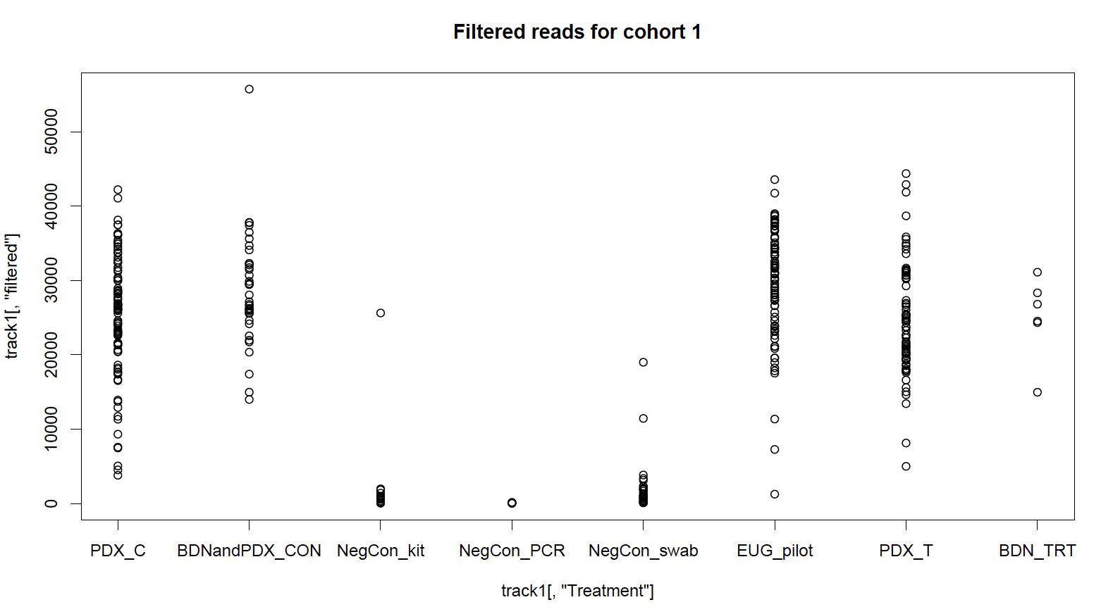
I had three types of negative controls: sterile DNA swabs which were processed to check for biological contamination in collection materials, kit controls where a blank extraction was run for each batch of extractions to test for biological contamination in extraction reagents, and PCR negative controls to check for DNA contamination of PCR reagents. In total, 90 control samples were sequenced, giving me unprecedented resolution to deal with contamination. Looking at the total number of sequences before and after my quality-analysis processing, I can see that the number of sequences in my negative controls reduces dramatically; they were low-quality in some way and might be sequencing artifacts. But, an unsatisfactory number remain after QA filtering; these are high-quality and likely come from microbial contamination.

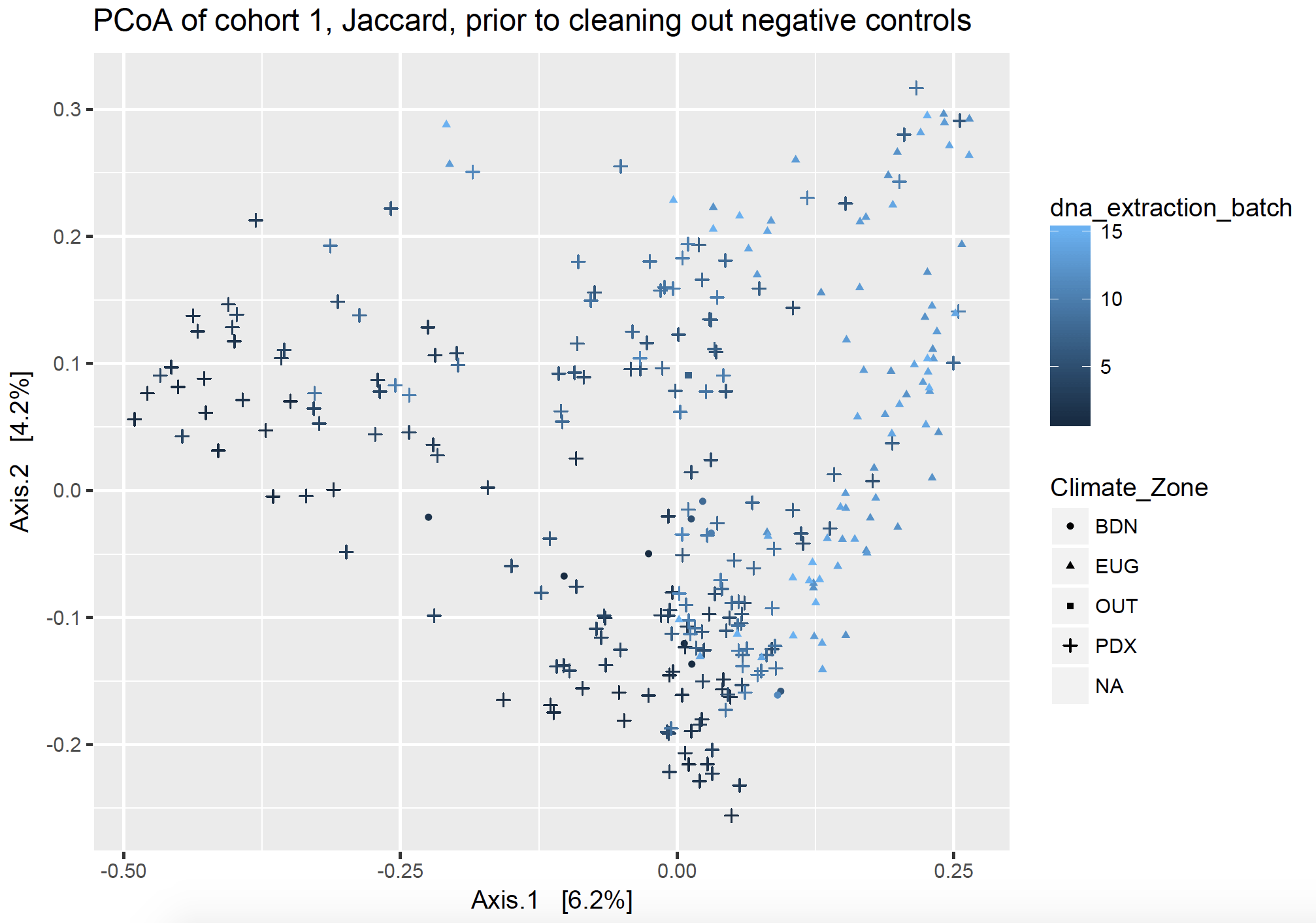
I wasn’t sure how I wanted to deal with each type of control. I came up with three approaches, and then looked at unweighted, non-rarefied ordination plots (PCoA) to watch how my axes changed based on important components (factors). What follows is a narrative summarize of what I did, but I included the R script of my phyloseq package workflow and workaround on GitHub.
Chapter 2
“In microbial ecology, preprints are posted on late November nights. The foreboding atmosphere of conflated factors makes everyone uneasy.”
Ordination plots visualize lots of complex communities together. In both ordination figures below, each point on the graph represents a dust sample from one house. They are clustered by community distance: those closer together on the plot have a more similar community than points which are further away from each other. The points are shaped by the location of the samples, including Bend, Eugene, Portland, along with a few pilot samples labeled “Out”, and negative controls which have no location (not pictured but listed as NA). The points are colored by DNA extraction batch.
Approach 1: Subtraction + outright removal
This approach subsets my data into DNA extraction batches, and then uses the number of sequences found in the negative controls to subtract out sequences from my dust samples. This assumes that if a particular sequence showed up 10 times in my negative control, but 50 times in my dust samples, that only 40 of those in my dust sample were real. For each of my DNA extraction batch negative control samples, I obtained the sum of each potential contaminant that I found there, and then subtracted those sums from the same sequence columns in my dust samples.

Approach 2: Total Removal
This approach removes any contaminant sequences that is found in ANY of the negative controls from ALL the house samples, regardless of which negative control was for which extraction batch. This approach assumes that if it a sequence was found as a contaminant in a negative control somewhere, that it is a contaminant everywhere.
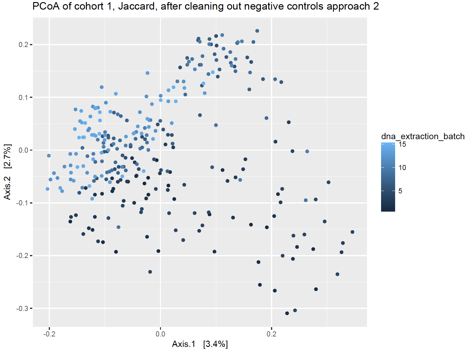
Additionally, I don’t favor throwing sequences out just because they were a contaminant somewhere, particularly for dust samples. Contamination can be situational, particularly if a microbe is found in the local air or water supply and would be legitimately found in house dust but would have also accidentally gotten into the extraction process.
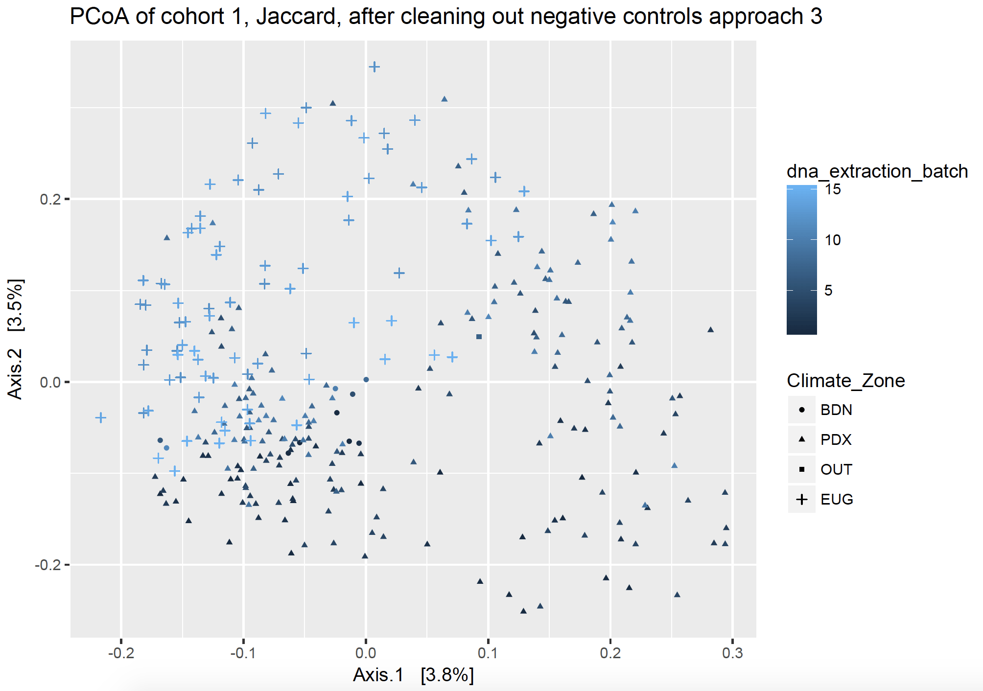
Approach 3: “To each its own”
This approach removes all the sequences from PCR and swab contaminant SVs fully from each cohort, respectively, and removes extraction kit contaminants fully from each DNA extraction batch, respectively. I took all the sequences of the SVs found in my dust samples and made them into a vector (list), and then I took all the sequences of the SVs found in my controls and made them into a different vector. I effectively subtracted out the contaminant SVs by name, but asking to find the sequences which were different between my two lists (thus returning the sequences which were in my dust samples but not in my control samples). I did this respective to each sequencing cohort and batch, so that I only remove the pertinent sequences (ex. using kit control 1 to subtract from DNA extraction batch 1).
Unlike its namesake, this tale has a happier ending.